Create real-time plots in Jupyter notebooks.
What is it?
It generalises Andreas Madsen's excellent python-lrcurve library for machine learning to produce visualisations for arbitrary functions in real-time.
pip install jupyterplot
Creating a simple real-time plot in a Jupyter notebook is as easy as easy as the following snippet:
from jupyterplot import ProgressPlot
import numpy as np

pp = ProgressPlot()
for i in range(1000):
    pp.update(np.sin(i / 100))
pp.finalize()
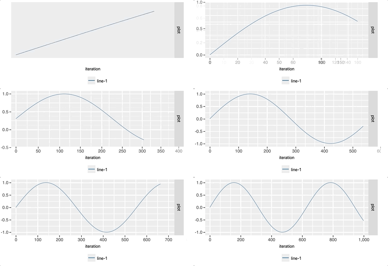
Note: The pp.finalize() statement is necessary to make the plots persistent between notebook sessions.
pp = ProgressPlot(x_lim=[0, 1000], y_lim=[-1.5, 1.5])
for i in range(1000):
    pp.update(np.sin(i / 100))
pp.finalize()

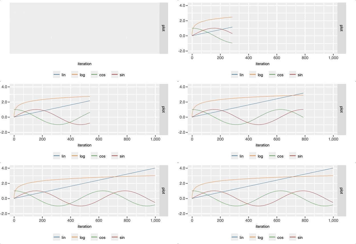
pp = ProgressPlot(line_names=["lin", "log", "cos", "sin"],
                  x_lim=[0, 1000],
                  y_lim=[-1, 4])

for i in range(1000):
    pp.update([[i / 250, np.log10(i + 1), np.cos(i / 100), np.sin(i / 100)]])
pp.finalize()

Note: The data is fed to pp.update() as a list of lists, where each sublist corresponds to the curves that are generated in each subplot.
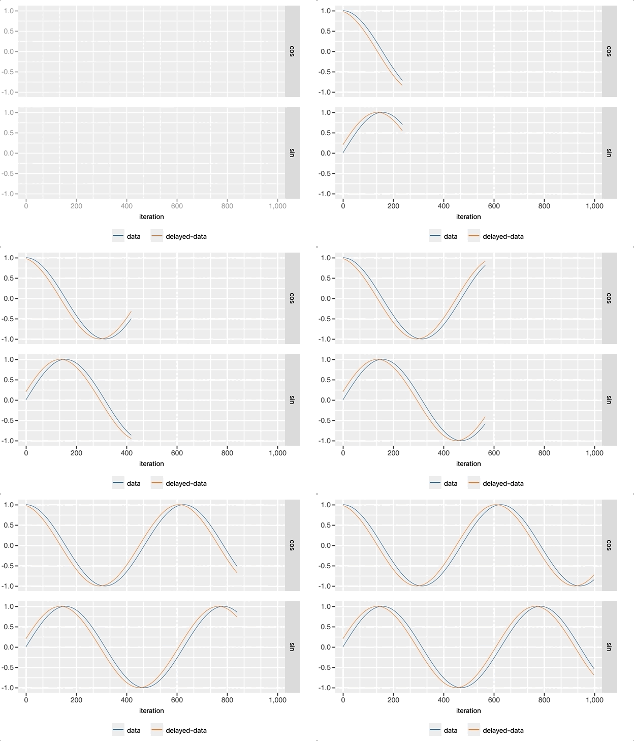
pp = ProgressPlot(plot_names=["cos", "sin"],
                  line_names=["data", "delayed-data"],
                  x_lim=[0, 1000],
                  y_lim=[-1, 1])

for i in range(1000):
    pp.update([[np.cos(i / 100), np.cos((i + 20) / 100)],
               [np.sin(i / 100), np.sin((i + 20) / 100)]])
pp.finalize()
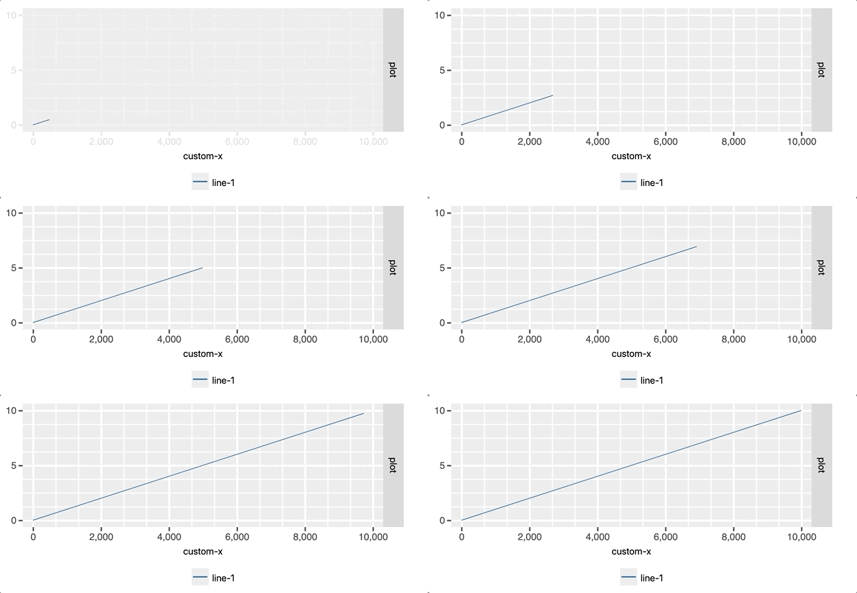
pp = ProgressPlot(x_iterator=False, x_label="custom-x", x_lim=[0, 10000], y_lim=[0, 10])
for i in range(1000):
    pp.update(10 * i, i / 100)
pp.finalize()
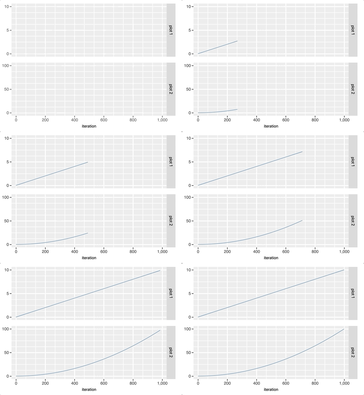
pp = ProgressPlot(plot_names=['plot 1', 'plot 2'], x_lim=[0, 1000], y_lim=[[0, 10],[0, 100]])
for i in range(1000):
    pp.update([[(i/100)], [(i/100)**2]])
Input format
Single plot, single line
If the progress plot consists of a single plot with a single line one can pass the y-updates as int or float.
Multiple plots, multiple lines
If multiple plots or lines are used, the y-updates can either be lists or dicts:
y_update_list = [[y_plot_1_line_1, y_plot_1_line_2],
                 [y_plot_2_line_1, y_plot_2_line_2]]

y_update_dict = {'plot_name_1': {'line_name_1': y_plot_1_line_1,
                                 'line_name_2': y_plot_1_line_2},
                 'plot_name_2': {'line_name_1': y_plot_2_line_1,
                                 'line_name_2': y_plot_2_line_2}}